
The Theory
Initial Motivation
This is mainly motivated by a problem regarding the Child and Family Service (CFS) in Saskatchewan, Canada. The CFS provides services to families to prevent child maltreatment. Also, in case a mere service provision does not guarantee child’s safety, CFS should provide out of home alternative care. According to the circumstances and child’s needs, a child may be placed in one of the following types of care:
- Foster Care (FC)
- Group Home (GH)
- Extended Family (EF)
- Other (OP)
There are (variable) costs associated to each of these care groups as well as those who are receiving services at home (SH) and a budget that is allocated to the CFS at the beginning of the fiscal year.
Many possible scenarios are imaginable for willing to change the trend in a certain group and/or their associated cost in a certain time frame. It might be easy to imagine how the bend in a trend may look like. It is very hard to imagine how this change affects other trends.
Of course one can remove these names from groups or assign other meanings and interpretations to the abstract groups and study a hypothetical scenario that fits this framework. Let us denote various groups at time \(t\) by \(G_1(t), G_2(t),\dots, G_n(t)\) and their associated cost by \(C_1(t), C_2(t),\dots, C_n(t)\). Also, denote the available budget at time \(t\) by \(B(t)\). To tackle this problem, we are going to make a few assumptions:
- The trend of the total capacity is invariant, meaning that although we may be able to assume changes in
each trend, but the total trend does not change. In symbols, if we introduce changes in certain group trends and they cause adjustments in other groups, i.e., \(G_i(t)\rightarrow G_i'(t)\), the following holds:
(1)¶\[\sum_{i=1}^n G_i(t) \approx \sum_{i=1}^n G_i'(t).\]
- The associated costs to groups are independent. A change in the cost of one group does not introduce changes
in the costs of other groups, unless it is forced that at the end of trial period, we have a non-negative budget residual.
Referring to the CFS problem, it should be clear that the number of children who require assistance from CFS in any form (i.e., services at home or kept at a place of safety) is independent from how CFS manages them (1). Also, adjustment in the costs of a certain group does not induce a change in the associates costs of other groups (2).
A Non-Deterministic Approach
Since we are interested in the general trends of various groups of items, it should be clear that the problem and hence any possible solutions mist likely live in a non-deterministic world. We are assuming that enough data points is provided over a consistent period of time for all groups \(G_1,\dots, G_n\) and their costs \(C_1,\dots, C_n\). Suppose that we are willing to use Regressors \(\mathcal{R}_1\) and \(\mathcal{R}_2\) to approximate trends of item groups and their costs, respectively, for a portion of time with available data, e.g, \([0, T]\) [We prefer not to use all existing data point as in some cases a part of data maybe affected by some protocols and policies that are not in effect anymore.]. In other words, the size of the item group $i$ at time $t$ can be approximated by
and for its cost
Suppose that the following changes are desirable:
and
A desirable change in the dynamics of the whole system that satisfies (2) and (3) should also introduce a minimal error in the system. We may use the values of \(\mathcal{R}_1[G_i](t)\) and \(\mathcal{R}_1[G'_i](t)\) to measure the introduced error. Among various options, we assume that the introduced error is measured by
which is \(\ell_2\) norm of the difference of two regressors over \([0, T]\).
The available budget at time \(t\) is \(B(t)-\sum_{i=1}^n(\mathcal{R}_1[G'_i](t)\times\mathcal{R}_2[C'_i](t))\). So, the residual of the budget after the end of trial period (\(t=T_f\)) is
which is typically desired to be maximized. Also, an alternative of (1) in terms of regressors should hold. So, we are interested in the optimum solutions of the following problem:
where the minimum is taken over all possible candidates for \(\mathcal{R}_1[G'_i]\) and \(\mathcal{R}_2[C'_i]\), \(i=1,\dots,n\).
Moreover, one may wishes that the residual at the end of trial period is non-negative. This adds the following extra constraint (5) to (4):
Enforcing Conditions on Regressors
To convince the regressors lean toward the values given on (2) and (3), we employ a Monte Carlo type of approach. Assuming that
to handle the constraint \(\mathcal{R}_1[G'_{i_j}](t_{i_j})=g_{i_j}\) we produce a random sample for a given period before and after time \(t_{i_j}\) drawn from the distribution \(\mathcal{N}(g_{i_j}, \sigma_i)\) and incorporate this artificial sample to our training data. This guarantees that \(\mathcal{R}[G'_{i_j}]\) leans toward \(g_{i_j}\) around time \(t=t_{i_j}\).
The strength of this bend is directly correlated to the size of the sample and the value of \(\sigma_i\). To make sure that the size of the sample is suitable, one can use a minimum number of sampled by default and use a ratio to estimate the maximum size of the sample [we will use the probability designated to determine confidence intervals as the default value for the ratio]. We repeat the same trick to handle the constraints of the form \(\mathcal{R}_2[C'_{i_k}](t_{i_k})=c_{i_k}\).
The set of constraints \(\mathcal{R}_1[G'_{i_j}](t_{i_j})=g_{i_j}\) determines the projected values of the corresponding items at time \(t=T_f\), trying to modify the ultimate values of these regressions for \(t=T_f\) clearly increases the value of \(\mathcal{E}\). So, we choose to relax the regressors to find their final values. For those indices \(i\not\in\{i_1,\dots,i_m\}\), we select candidate values \(\tilde{g}_i\) such that
This reduces solving (4) to finding best candidates for \(\tilde{g}_i\), \(i\not\in\{i_1,\dots,i_m\}\) that minimizes the objective of (4) and satisfies (6). Algorithm summarizes this procedure.
Example
To see the algorithm in action we use the CFS’ data with hypothetical data for the corresponding costs and budget. Next table provides a few samples from data. The ds ranges from January 1th, 2015 to January 1th, 2019. We chose the last year of the data to base the analysis on and project trends for January 11th, 2021.
| ds | FC | GH | EF | OP | SH | FCc | GHc | EFc | OPc | SHc |
|---|---|---|---|---|---|---|---|---|---|---|
| 2018-08-30 | 924 | 780 | 2816 | 880 | 1969 | 5.97549 | 6.48204 | 1.98615 | 2.86382 | 1.77176 |
| 2017-12-21 | 927 | 712 | 2816 | 885 | 1863 | 4.63028 | 5.83286 | 2.42853 | 2.68884 | 1.60908 |
| 2016-10-13 | 968 | 666 | 2536 | 876 | 1660 | 4.06597 | 4.22486 | 1.77068 | 1.82547 | 1.34815 |
| 2017-06-08 | 993 | 744 | 2655 | 854 | 1802 | 4.89702 | 4.77482 | 1.39608 | 1.91099 | 0.931255 |
| 2015-12-17 | 948 | 565 | 2515 | 827 | 1729 | 3.17565 | 3.0835 | 0.831563 | 1.85582 | 1.04643 |
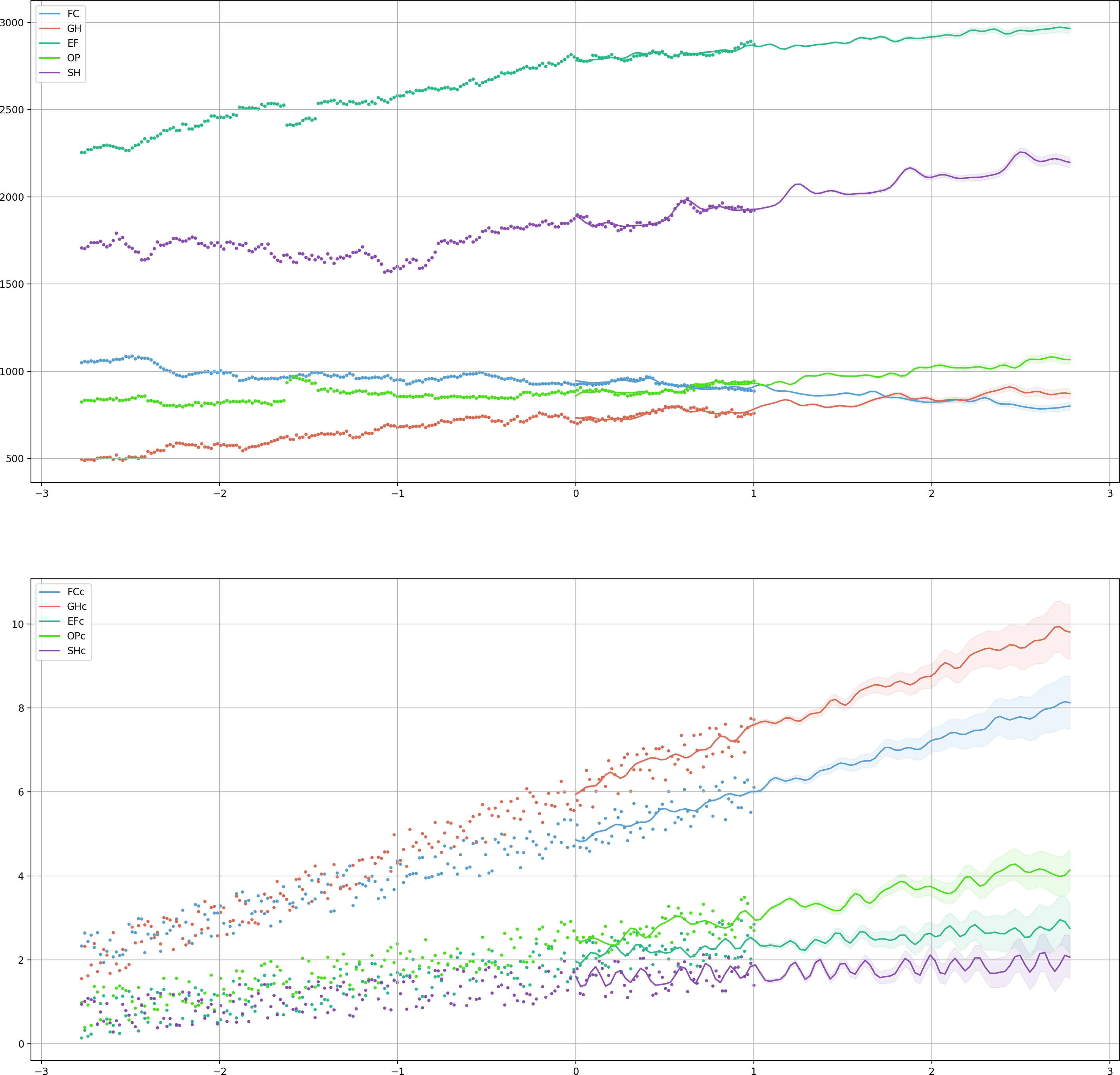
The following figure shows the data points and their trends estimated based on a Fourier transform.
Then we set the following constraints for points at time in future:
- 650 for G at January 1th, 2021
- 700 for FC at January 1th, 2021
- 6.0 for FCc at January 1th, 2020
- 8.0 for GCc at January 1th, 2021
- 2.5 for EFc at January 1th, 2020
- 3.5 for OPc at January 1th, 2020
Assuming that the DataFrame df is already set, the following piece of code sets up and runs the analysis:
# initiated df
pairs= [('FC', 'FCc'), ('GH', 'GHc'), ('EF', 'EFc'), ('OP', 'OPc'), ('SH', 'SHc')]
# define regressors
from NpyProximation import HilbertRegressor
from numpy import sin, cos, exp
deg = 5
skip = 1
l = 0.1
base = [lambda x: 1., lambda x: x[0]] + \
    [lambda x, l=l, _=_: sin(_*x[0]/l) for _ in range(1, deg+1, skip)] + \
    [lambda x, l=l, _=_: cos(_*x[0]/l) for _ in range(1, deg+1, skip)]
regressor = HilbertRegressor(base=base)
# initialize
s_date = datetime(year=2018, month=1, day=1)
instance = InventoryOpt(df, date_fld='ds', units_costs=pairs, start_date=s_date,
            num_intrvl=(0., 1.), projection_date=datetime(year=2021, month=1, day=1),
            c_limit=.95)
instance.set_unit_count_regressor(regressor)
instance.set_cost_regressor(regressor)
instance.fit_regressors()
instance.plot_init_system().savefig('init.png', dpi=200)
instance.budget = lambda t: 30000-22000*exp(-t-1.)
# constraints
instance.constraint('GH', 650, datetime(year=2021, month=1, day=1))
instance.constraint('FC', 700, datetime(year=2021, month=1, day=1))
instance.constraint('FCc', 6., datetime(year=2020, month=1, day=1))
instance.constraint('GHc', 8., datetime(year=2021, month=1, day=1))
instance.constraint('EFc', 2.5, datetime(year=2020, month=1, day=1))
instance.constraint('OPc', 3.5, datetime(year=2020, month=1, day=1))
# run
instance.adjust_system(tbo='b')
fig = instance.plot_analysis()
After running the analysis, the followin figure would be the outcome.
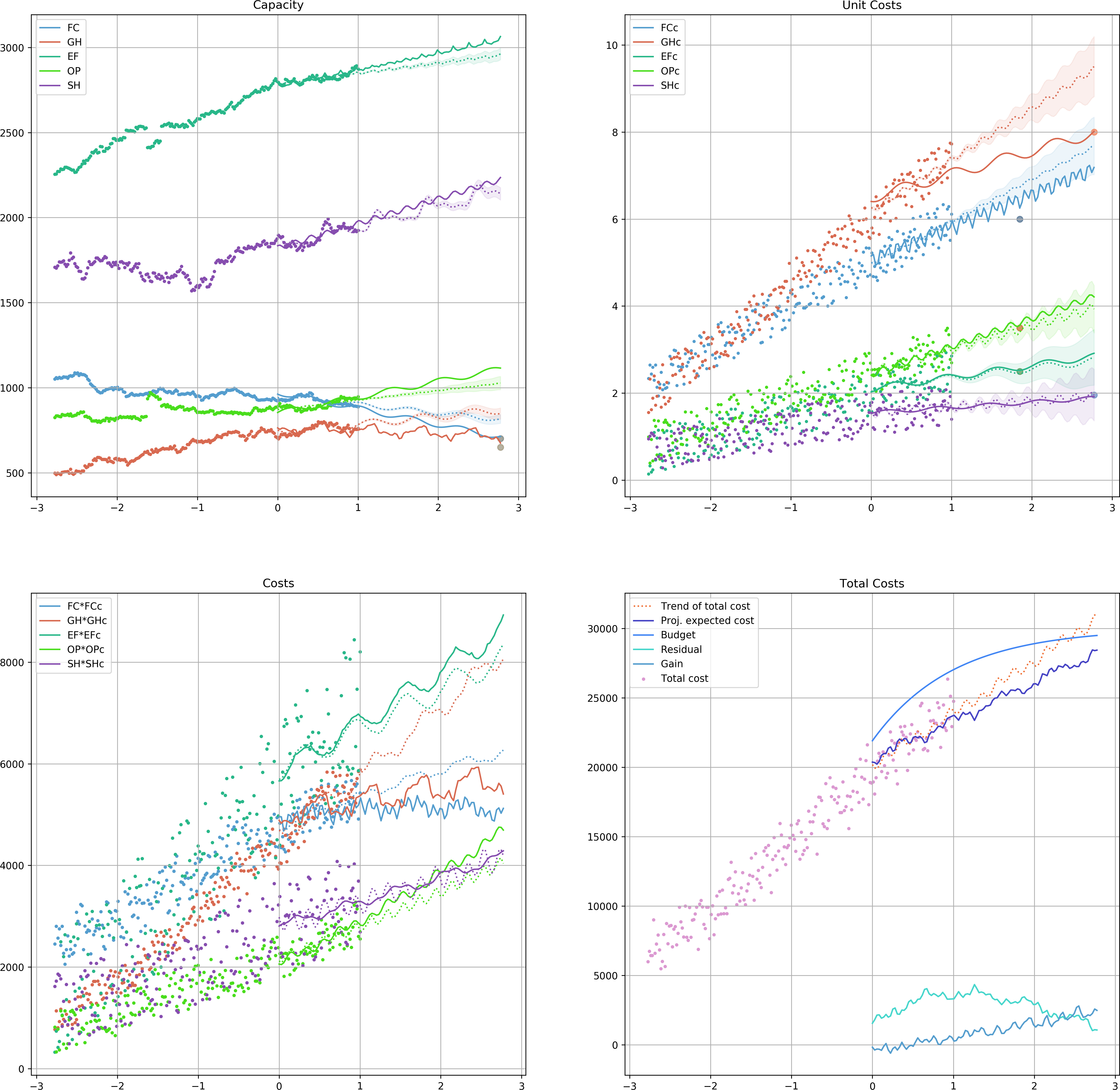
Note that in some cases the solver was not able to perfectly match the suggested value at the specific time. This is due to the stochastic nature of the problem and the provided solution.